SEGGER’s J-Trace PRO streaming trace probe and Ozone debugger make a great team. One highlight of this symbiotic relationship is the Timeline window. It allows users to correlate and visualize data sampling, current consumption, and program execution in one combined signal plot. This article takes a closer look at this functionality.
The Ozone Timeline window
Let’s take a quick look at the three elements of the Timeline window in Ozone. The timeline’s Data pane displays the graphs of sampled variables and expressions. The Power pane displays the target’s power consumption. The Code pane displays the visual representation of the program’s call stack, generated from traced program execution.
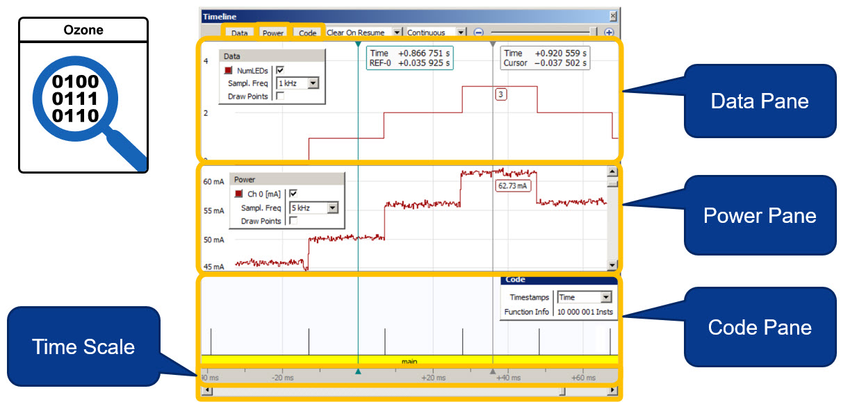
All panes in the timeline window share a common timescale. This enables users to compare the target’s power consumption against code execution, or to observe the state of selected data at a particular point in program execution.
Setting up the hardware
To see this in action, we can use the SEGGER Ozone debugger, a SEGGER J-Trace PRO, plus a target board that is suitable to be powered by J-Trace PRO, such as one of SEGGER’s Trace Reference Boards.
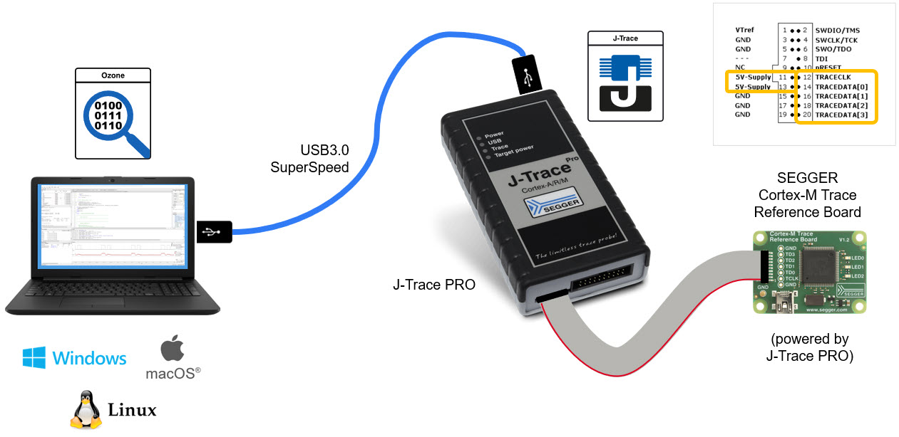
The target device needs to have the Embedded Trace Macrocell (ETM) or Program Trace Macrocell (PTM) plus the associated Trace Data and Trace Clock pins.
Note that you can also connect to the J-Trace PRO via Gigabit Ethernet.
Loading the example project
As the Software project, we can use the Ozone J-Trace PRO Tutorial Project from the SEGGER website. The project creates two embOS RTOS tasks that toggle two LEDs at different intervals.
After downloading and running the project, we can graph the values of two global variables, Count 1 and Count 2, in the Data Pane. We can also see the current consumption of the board in the Power Pane. The current consumption varies, depending on how many LEDs are turned at any given time.
After we halt the program execution, the code pane in the timeline window gets updated.
Analyzing the current consumption in correlation with program execution
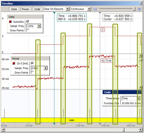
Now we can zoom into the timeline and see how the change in current consumption correlates with the task switches in the code.
We can see that whenever one of the two tasks turns an LED on or off, the current jumps or drops by about 6 mA shortly afterwards.
Zooming even closer into the details of the task switch shows how the embOS RTOS switches from the Idle Task to one of the two tasks toggling the LEDs and then switches back to the Idle Task.
Observed changes in current by about 12 mA are caused by both tasks being executed back-to-back and both turning their respective LEDs on or off.
In this case we see three task switches happening: From the Idle Task to the higher-priority task, then to the lower-priority task, and then back to the Idle Task.
Interesting to note is that the selected row in the Power Sampling Window is synchronized with the sample cursor of the Timeline Window.
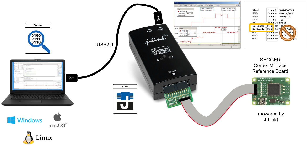
You can also use the Ozone Timeline Window with a SEGGER J-Link, without instruction trace. However, in this case only the Data Pane and the Power Pane will be populated.
Summary
As we saw, the timeline window in SEGGER’s Ozone debugger allows you to correlate and visualize data sampling, current consumption, and program execution in one combined signal plot.
Of course, let’s not forget about Ozone’s capability to display the complete instruction trace history as well as live Code Coverage and Code Profiling information.
To learn more about Ozone, J-Trace PRO, or any of our other hardware or software products, please visit www.segger.com.
Thanks for reading!